Master Google Sheets with 10 essential steps for productivity, including the top 30 Google Sheet Short keys and functions, Check below!
About Google Sheet
Google Sheets is an efficient online application for creating spreadsheets. This belongs to the Google Drive productivity suite, which provides comparable functionality to spreadsheet software like Microsoft Excel.
Google Sheets is a great online tool for creating, editing, and collaborating on spreadsheets. It offers many useful features for organizing and analyzing data, including formulas, charts, and conditional formatting. You can easily share your work with others for real-time collaboration.

10 Basic Steps to Learn Google Sheets
- Access Google Sheets: Go to the Google Sheets website (sheets.google.com) and sign in to your Google account. You can create one for free if you don’t have an account.
- Create a new spreadsheet: Click on the “+ New” button to create a new spreadsheet. Alternatively, you can open an existing spreadsheet from Google Drive.
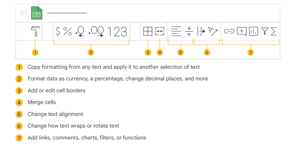
- Familiarize yourself with the interface: Take a few moments to explore the different elements of the Google Sheets interface, such as the menu bar, toolbar, formula bar, and the main grid where you enter data.
- Enter data: Start by entering data into cells. Click on a cell and type in your desired content. Press Enter to move to the next cell.
- Format your data: Google Sheets provides various formatting options to customize the appearance of your data. You can change font styles, colours, alignment, and cell borders to make your spreadsheet more visually appealing.
- Use basic formulas: Google Sheets supports a wide range of formulas and functions that allow you to perform calculations on your data. Begin with simple procedures like addition, subtraction, multiplication, and division to get familiar with the formula syntax.
- Insert and delete rows/columns: Learn how to insert and delete rows or columns to reorganize your data. Right-click on the row/column headers and select the appropriate option from the context menu.
- Conditional formatting: Conditional formatting allows highlighting cells based on specific conditions. For example, you can set a rule to highlight all cells with values above a certain threshold in a different colour.
- Create charts: Google Sheets makes it easy to visualize your data using various chart types, such as bar graphs, pie charts, and line charts. Select the data you want to include in the chart, click the “Insert” menu, and choose the desired chart type.
- Collaborate and share: Google Sheets is designed for collaboration so that you can work on spreadsheets with others in real-time. Use the “Share” button to invite collaborators and set their permissions to view, comment, or edit the spreadsheet.
Create your first spreadsheet
To Create or import a spreadsheet follow the steps given below,
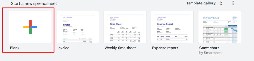
- To Create first click on the Google Apps icon select ‘Sheets’, and click on ‘blank’, for more clarity check the below mention image below,
If you have existing files, you can import and convert them to Docs, Sheets, or Slides.
- Go to Drive.
- Click Newand thenFile Upload.
- Choose the file you want to import from your computer to add it to Drive.
- In the Upload Complete window, click Show file location.
- Right-click the file and select Open with>Google Sheets.
To Organize data
Add rows, columns, and cells:
- Select the row, column, or cell near where you want to add your new entry.
- Right-click the highlighted row, column, or cell>Insert>choose where to insert the new entry.
Delete, clear, or hide rows and columns
- Right-click the row number or column letter.
- Click Delete, Clear, or Hide.
Delete cells
- Select the cells
- Right-click>Delete cells>Shift left or Shift up.
Move rows or columns: Select the row number or column letter and drag it to a new location.
- Move cellsSelect the cells.
- Point your cursor to the top of the selected cells until a hand appears.
- Drag the cells to a new location.
Group rows or columns
- Select the rows or columns.
- Click Data>Group rows or Group columns.
Freeze header rows and columns: Keep a row or column in the same place as you scroll through your spreadsheet. On the menu bar, click View>Freeze and choose an option.
Add formulas or functions
- Open a spreadsheet.
- Type an equal sign (=) in a cell and type in the function you want to use.
Note: You may see suggested formulas and ranges based on your data.
A function help box will be visible throughout the editing process to provide you with a definition of the function and its syntax, as well as an example for reference.
To learn more about formulas and functions check this tutorial.
Google Sheets Cheat Sheet
Work with Functions
| AVERAGE | Statistical Returns the numerical average value in a dataset, ignoring text. |
| AVERAGEIFS | Statistical Returns the average of a range that depends upon multiple criteria. |
| CHOOSE | Lookup Returns an element from a list of choices based on the index. |
| COUNT | Statistical Returns the count of the number of numeric values in a dataset. |
| COUNTIF | Statistical Returns a conditional count across a range. |
| DATE | Date Converts a provided year, month, and day into a date. |
| FIND | Text Returns the position at which a string is first found within the text. |
| GETPIVOTDATA | Text Extracts an aggregated value from a pivot table that corresponds to the specified row and column headings. |
| IF | Logical Returns one value if a logical expression is true and another if it is false. |
| INDEX | Lookup Returns the content of a cell, specified by row and column offset. |
| INT | Math Rounds a number down to the nearest integer that’s less than or equal to it. |
| LOOKUP | Lookup Looks through a row or column for a key and returns the value of the cell in a result range located in the same position as the search row or column |
| MATCH | Lookup Returns the relative position of an item in a range that matches a specified value. |
| MAX | Statistical Returns the maximum value in a numeric dataset. |
| MIN | Statistical Returns the minimum value in a numeric dataset. |
| NOW | Date Returns the current date and time as a date value. |
| ROUND | Math Rounds a number to a certain number of decimal places according to standard rules. |
| SUM | Math Returns the sum of a series of numbers and/or cells. |
| SUMIF | Math Returns a conditional sum across a range. |
| TODAY | Date Returns the current date as a date value. |
| VLOOKUP | Lookup Searches down the first column of a range for a key and returns the value of a specified cell in the row found. |
Click here to learn more…
Top 30 Google Sheet Short Keys
- Move to the beginning of the sheet: Ctrl + Home
- Move to the end of the sheet: Ctrl + End
- Select the entire column: Ctrl + Spacebar
- Select the entire row: Shift + Spacebar
- Select the entire sheet: Ctrl + A
- Insert a new sheet: Shift + F11
- Insert a new row or rows: Ctrl + Shift + + (plus sign)
- Insert a new column or columns: Ctrl + Shift + + (plus sign)
- Delete the selected row or rows: Ctrl + –
- Delete the selected column or columns: Ctrl + –
- Undo the last action: Ctrl + Z
- Redo the last undone action: Ctrl + Y
- Copy the selected cells: Ctrl + C
- Cut the selected cells: Ctrl + X
- Paste the copied or cut cells: Ctrl + V
- Apply bold formatting: Ctrl + B
- Apply italic formatting: Ctrl + I
- Apply underline formatting: Ctrl + U
- Insert the sum function: Alt + Shift + =
- Insert the average function: Alt + Shift + A
- Insert the current date: Ctrl + ;
- Insert the current time: Ctrl + Shift + :
- Insert a hyperlink: Ctrl + K
- Format cells as currency: Ctrl + Shift + 4
- Format cells as a percentage: Ctrl + Shift + 5
- Insert a line break within a cell: Alt + Enter
- Toggle between displaying formulas and values: Ctrl + ` (backtick)
- Open the Find and Replace dialog: Ctrl + H
- Open the Filter menu: Ctrl + Shift + L
- Open the Explore panel: Alt + Shift + X
FAQs
What is Google Sheet Duplicate Formula?
Customize your duplicate checking formula by entering it in the Value or Formula bar. For example: you’re looking for duplicates in cells X2:X15, so the custom formula is =COUNTIF($X$2:$X$15, X2)>1. If your duplicates are in a different data range (for example, Y2:Y15), your custom formula would be =COUNTIF($Y$2:$Y$15,Y2)>1
How to Convert the Google Sheet to PDF?
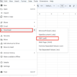
Follow the below-mentioned steps:
1. Select File Tab
2. Select Download
3. Finally Click on the PDF button and download the desired file.